How To Do Filter Sum In Excel

09 Oct, 2021

Normally the AutoSum icon inserts a SUM function. Click the Sort Filter drop down from the Editing group.

Excel Tutorials Top Ten Excel Functions You Have To Know Excel 2019 If Vlookup Sum Pmt Youtube Excel Tutorials Microsoft Excel Tutorial Excel

You can use the AutoSum icon after applying a filter.

How to do filter sum in excel. To sum the filtered values in column C based on the criteria please enter this formula. Thats contrary to the usual practice of adding parameters to the end when a function is based on a previous version. If you are hiding rows manually ie.

If you use SUM function for it it will show you the SUM of th. Select the data to be filtered and then on the Data tab click Filter. It should open a window where you can select Filter and then Value Filters.

SUMIF range criteria sum_range The SUMIF function syntax has the following arguments. SUBTOTAL9 F5F14 which returns the sum 954 the total for the 7 rows that are still visibleIf you are hiding rows manually ie. Change the formula from SUM C2C50 to SUBTOTAL 9C2C50 and see the magic.

Blank and text values are ignored. Once we do that we will get the Output cell filtered sum as 190 as shown below. SUM Filtered Data Using SUBTOTAL Function.

The solution is much easier than you might think. How to filter by sum values pivot table colbrawl Try by right-clicking on any of the row labels of your pivot table. Simply click AutoSum-- Excel will automatically enter a SUBTOTAL function instead of a SUM.

Click Home from the Ribbon. The solution to our problem lies in using the SUBTOTAL Function. Just organize your data in table Ctrl T or filter the data the way you want by clicking the Filter button.

Excel sum of visible rows. SumIF has filtercriteria first followed by the range to add up. Display workbook in Excel containing data to be filtered.

You may sum filtered cells while excluding those with error values AGGREGATE or SUBTOTAL by using AGGREGATE9 3 B2B1000. A SUBTOTAL formula will be inserted summing only the visible cells in. Here we have selected YELLOW as shown below.

After that select the cell immediately below the column you want to total and click the AutoSum button on the ribbon. The formula used is. Learn how to SUM only filtered data in Excel.

SUBTOTAL9 F5F14 which returns the sum 954 the total for the 7 rows that are still visible. Here you can set the filter to your liking. In the example shown a filter has been applied to the data and the goal is to sum the values in column F that are still visible.

This function will ignore rows hidden by the Filter command. The range of cells that you want evaluated by criteria. The formula used is.

When you apply a filter and then use AutoSum Excel will insert a SUBTOTAL function instead. Now apply the filter in the top row by pressing Ctrl Shift L. Click anywhere in the data set.

The first thing you will need to do is apply Filter to your data and then be sure to have the data filtered BEFORE trying to SUM the range. When you filter data getting the SUM of only the visible part of the data can be a challenge. In the example shown a filter has been applied to the data and the goal is to sum the values in column F that are still visible.

If you filter after applying the SUM function you will still see the total including the data hidden by the filter. If you need to sum filtered cells while also excluding those that dont satisfy a criteria you may use the combination of SUBTOTAL and OFFSET in a SUMPRODUCT formula. Cells in each range must be numbers or names arrays or references that contain numbers.

Go to Filter by Color from the drop-down menu of it. Sum visible rows in a filtered list Exceljet. SUM has the range to be added first obviously so people rightly expect SumIF to put the criteria after that.

In filtered list SUBTOTAL always ignores values in hidden rows regardless of the function argument. This tutorial will cover two quick and easy ways to ensure you get the SUM of only filtered data in ExcelTimes. SUMPRODUCTSUBTOTAL3OFFSETB6B19ROWB6B19-MINROWB6B191 B6B19NellyC6C19 B6B19 contains the criteria that you want to use the text Nelly is the criteria and C6C19 is the cell values you want to sum and then press Enter key to return the result as.

Sum Columns Or Rows Of Numbers With Excel S Sum Function Excel Excel Shortcuts Sum

How To Sum Filtered Data Using Subtotal Function In Excel Exceldatapro Excel Function Data

Multi Level Pivot Table In Excel Excel Pivot Table Microsoft Excel

How To Use Filter Formula In Excel Excel Tutorials Excel Tutorials Excel Excel Formula

Alt Select The Range With The Numbers You Want To Total And Press Enter Column Sum Expense Sheet

Set Up The Following Ranges Similar To What You Would Use For An Advanced Filter A Database Range A Criteria Range In This Example The Sum Ms Office Excel

Microsoft Excel Remove Grand Totals And Subtotals From Pivot Tables Microsoft Excel Excel Tutorials Excel

Add A Search Box To The Slicer To Filter It Quickly Pivot Table Keyboard Shortcuts Workbook

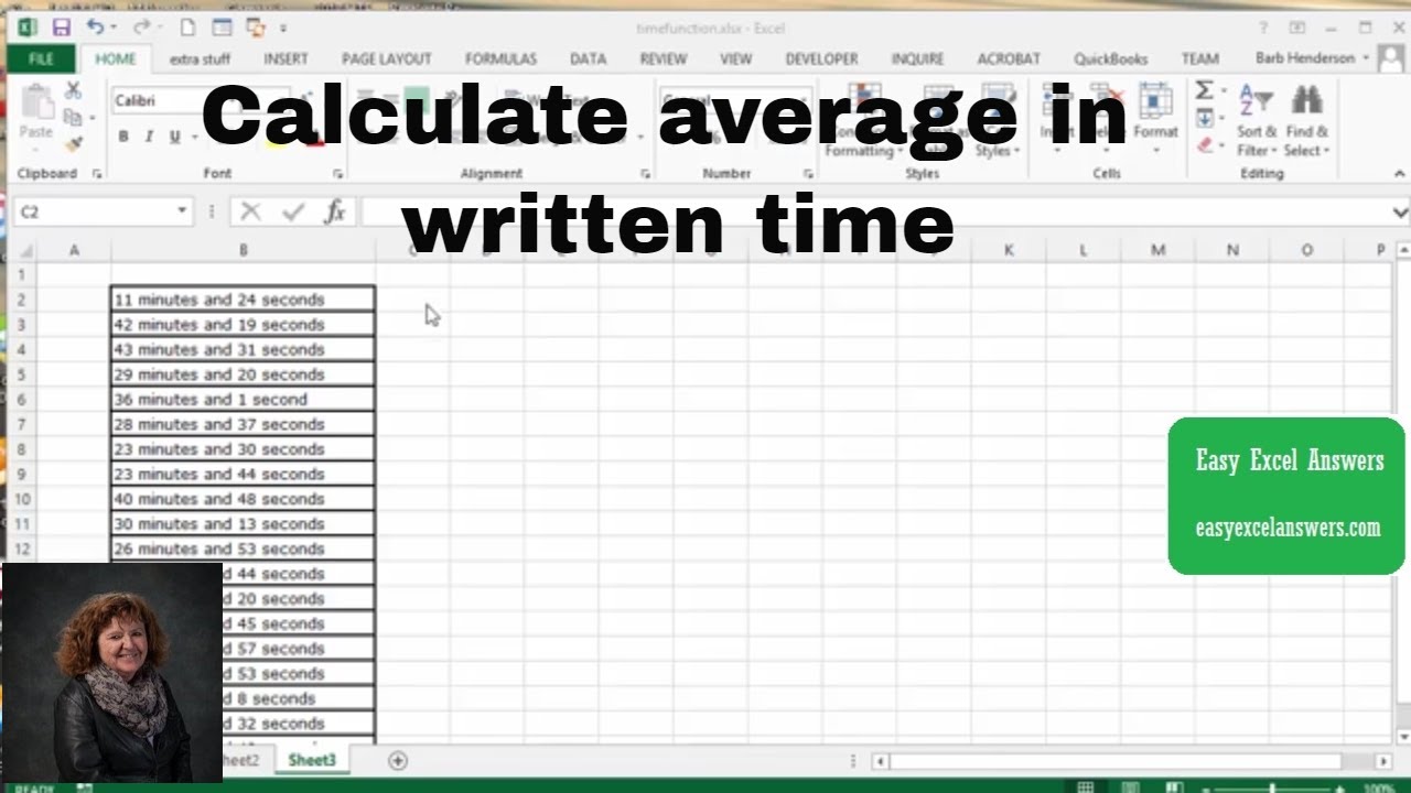
How To Calculate The Average Of Time When The Time Is Written In English Marketing Words Daily Calendar Template Social Media Content Calendar

Creating Strong Data And Filter Function Microsoft Excel Is Part Of The Microsoft Office Package Of Productivity Software It S Al Basic Math Make Charts Excel

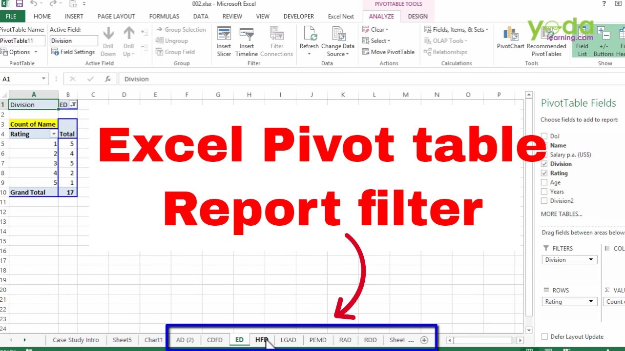
Excel Pivot Table Report Filter Advanced Excel Youtube Pivot Table Excel Tutorials Pivot Table Excel

Set Up The Following Ranges Similar To What You Would Use For An Advanced Filter A Database Range A Criteria Range In This Example Excel Workbook New Names