How Do I Add A Total To A Waterfall Chart In Excel
Waterfall charts in excel waterfall chart in excel easiest 5 waterfall charts tools how to create a waterfall chart in excel how to create waterfall charts in excel. Waterfall charts otherwise known as bridge charts illustrate upward and d.
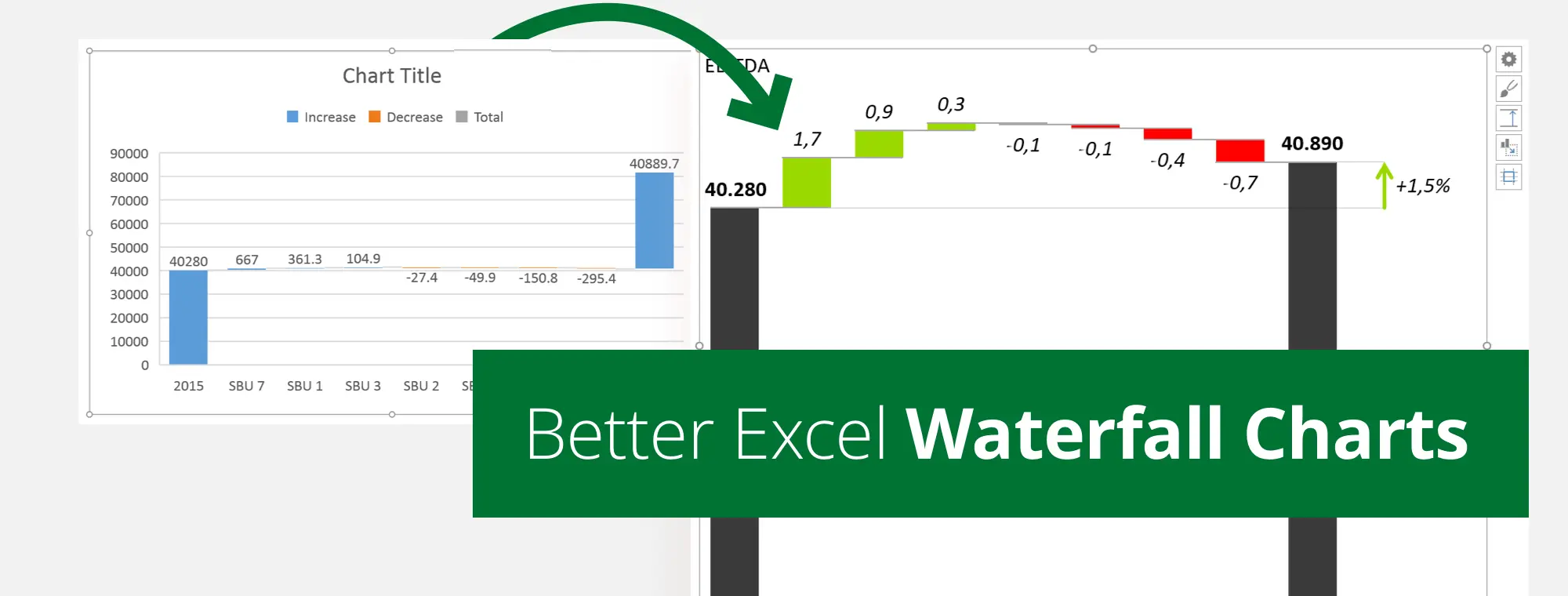
The New Waterfall Chart In Excel 2016 Peltier Tech
Waterfall charts also called bridge graphs are an excellent way to summarize a variance analysis for business rev.
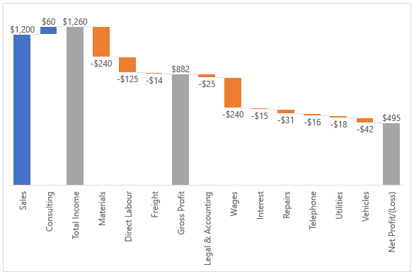
How do i add a total to a waterfall chart in excel. When I place the measure on a table or grid it shows the total properly but when I use the waterfall chart it shows the total as 1525540. Select the stacked column chart and click Kutools Charts Chart Tools Add Sum Labels to Chart. How to create a waterfall chart in Excel.
If you have an earlier version of Excel you can use an alternative method to plot. If so well done. Insert tab Line chart.
Next select D4 in the Up column and enter this. Go to the Insert tab. Your chart should now look like this.
Double-click a data point to open the Format Data Point task pane and check the Set as total box. As youll see you should only use the easy right-click option. Its faster and less cumbersome than the formatting pane.
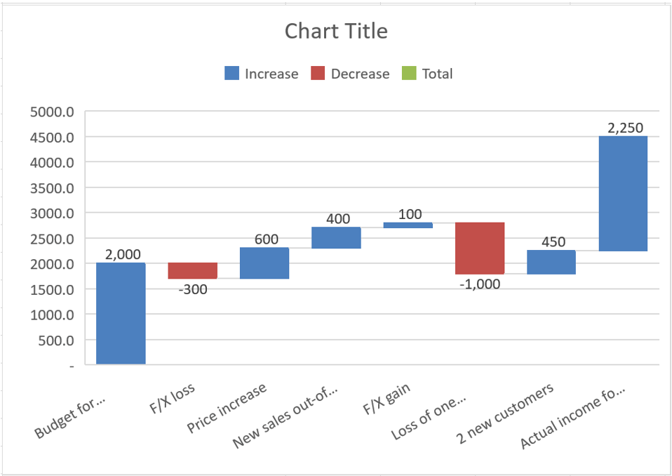
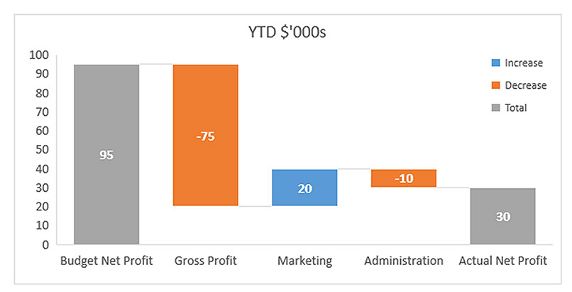
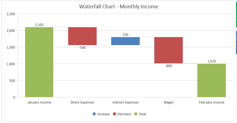
Increase Decrease and Total. So in the waterfall chart I should see 15 then an increase should show from the 15 to the 25 then a decrease should show from 25 to 5. The right-click menu and the formatting data point settings within the formatting pane.
Now select the entire data range go to insert charts column under column chart select Stacked column as shown in the below screenshot. It will give you three series. Creating Manual Excel Waterfall Charts Step 1.
Select the data range that you want to create a waterfall chart based on and then click Insert Insert Waterfall Funnel Stock Surface or Radar Chart Waterfall see screenshot. Then all total labels are added to every data point in the stacked column chart immediately. Start subtotals or totals from the horizontal axis.
Select data in cells A5A19 then hold CTRL and select cells C5E19 Step 2. Highlight all the data A1B13. If you dont see these tabs click anywhere in the waterfall chart to add the Chart Tools to the ribbon.
Drag the fill tool to the end of the column to copy the formula. Now we need to convert this stack chart to a waterfall chart with the below steps. Select the Insert Waterfall Funnel Stock Surface or Radar Chart button.
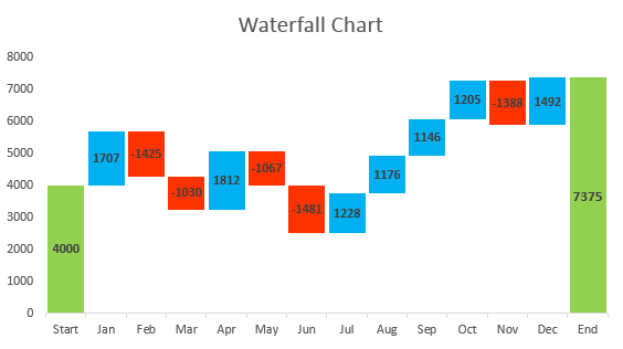
Firstly make five columns Time Base Decrease Increase and Net Cash. Navigate to the Insert tab and click the Waterfall chart button. Click in the formula bar type an sign then click on the cell that contains the label.
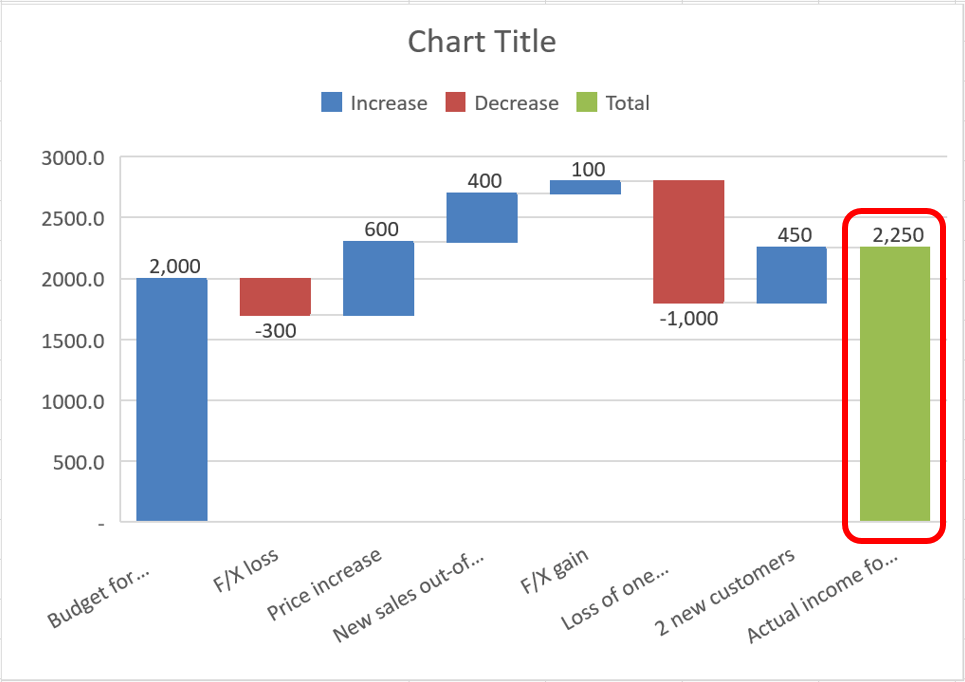
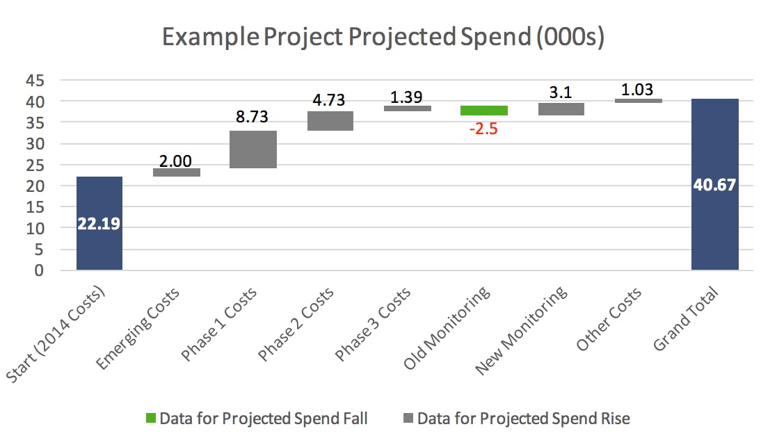
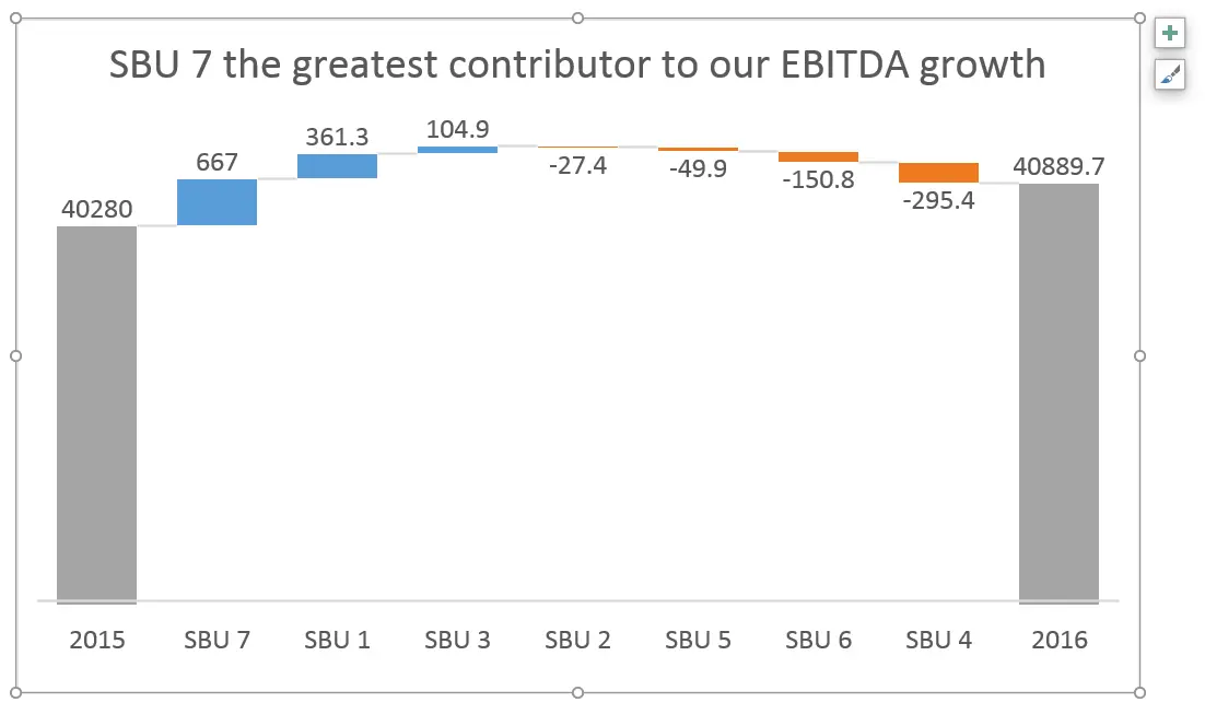
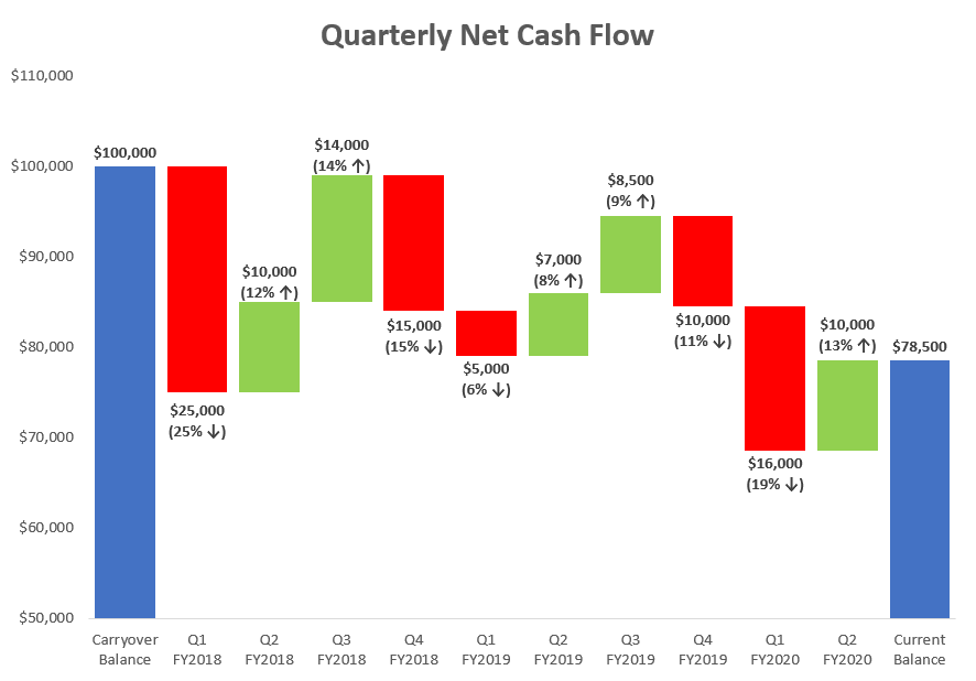
For some categories changes are positive and in some cases they are negative. If your data includes values that are considered Subtotals or Totals such as Net Income you can set those values so they start on the horizontal axis at zero and dont float. Dont click so much as the cursor starts blinking in the label.
Start subtotals or totals from the horizontal axis If your data includes values that are considered Subtotals or Totals such as Net Income you can set those values so they start on. Next you should set the net total income value to start on the horizontal axis at. Creating the chart.
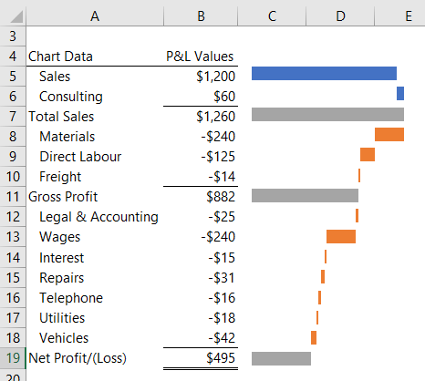
And now a chart has been inserted into the sheet see screenshot. In this example were using a simple expenses and income table. IF E40 E40 Use the fill tool to drag the formula down to the end of the column again.
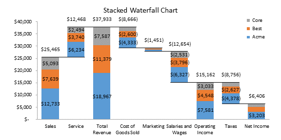
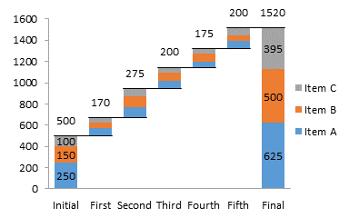
Now your Excel waterfall chart should look like this. To plot this chart simply select the cells B3. How To Create A Stacked Bar Waterfall Chart In Excel.
Select the source data and click Insert Insert Column or Bar Chart Stacked Column. There are two easy ways to set totals in Excel waterfall charts. To use the new Excel 2016 Waterfall Chart highlight the data area including the empty cell right above the categories and Insert Waterfall Chart.
At this point you will see the first two but not the Total. You will get the chart as below. Select each label two single clicks one selects the series of labels the second selects the individual label.
Insert the chart. C16 and click on the waterfall chart to the plot. Select the data you want to create the waterfall chart from.
This short tutorial video demonstrates how to build a waterfall chart in Excel. Written by Kupis on May 28 2020 in Chart. The New Waterfall Chart In Excel 2016 Peltier Tech.
How To Create Waterfall Charts In Excel

How To Set The Total Bar In An Excel Waterfall Chart Analyst Answers
How To Create Waterfall Chart In Excel 2016 2013 2010
Excel Waterfall Charts My Online Training Hub
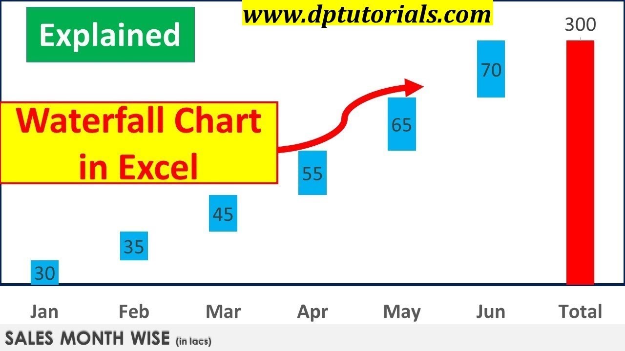
Excel Tricks How To Create Waterfall Chart In Excel Excel Graphs Excel Tips Dptutorials Youtube
Create A Waterfall Chart In Excel 2016 Intheblack
How To Create Waterfall Charts In Excel
Stacked Waterfall Chart Microsoft Power Bi Community


Why Would I Use A Cascade Waterfall Chart Mekko Graphics
Tutorial Create Waterfall Chart In Excel
Excel Waterfall Charts Bridge Charts Peltier Tech
Building A Waterfall Chart In Excel Trexin Consulting
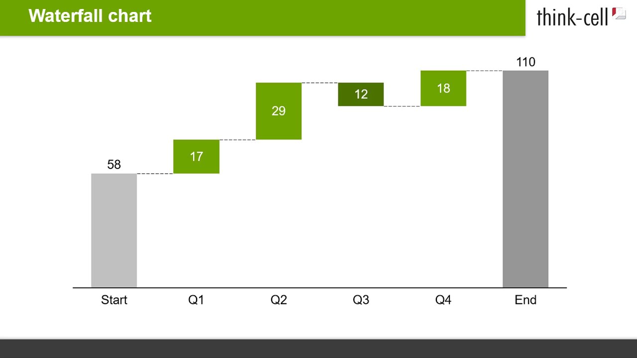
Waterfall Chart Think Cell Tutorials Youtube
Excel Waterfall Chart How To Create One That Doesn T Suck
Excel Waterfall Charts My Online Training Hub

Create Waterfall Or Bridge Chart In Excel
Create An Excel 2016 Waterfall Chart Myexcelonline
Excel Waterfall Chart How To Create One That Doesn T Suck
How To Create A Waterfall Chart In Excel Automate Excel